CPSC 322: Introduction to Artificial Intelligence

Day 1

• What is AI:

  • Machine think like human
  • Machine think rationally

• Thinking and acting like humans

• Model cognitive functions of humans

  • Humans only example of intelligence

• Turing test: use operational definition => consider intelligent when can’t tell between computer or human

• Downside:

  • don’t have detailed model of people’s mind yet
  • trickey/lying involved

• Thinking and acting rationally

  • Rationally: abstract ideal of intelligence
  • Syllogism: argument structures that always yield correct conclusions given correct premises => logic + probabilistic reasoning
  • Correct reasoning is enough?
  • AI as building agents: artifacts that are able to think and act rationally in their environments
    • Rationality more cleanly defined than humans
    • Agents can: answer query, plan actions, solve complex problems

• What is an agent (does not need all)

  • Situated in an environment
  • Make observations
  • Able to act
  • Has goals or preferences
  • Prior knowledge or beliefs, way to update beliefs based on new experiences

Day 2

What do we need to represent

• Environment/world
  • states/possible worlds
• how the world works => rules
  • Constraints
  • Casual relationships
  • Action preconditions and effects

Corresponding reasoning tasks and problems

• Constraint satisfaction (static): find a state that satisfies some set of constraints
• Answering queries (static)
  • Is a given proposition true/likely given what is known
• Planning (sequential): choose actions to reach goal state or maximize utility

Representation And reasoning system

• Sensing uncertainty => can agent fully observe current state of world or is there uncertainty in what we observe
• Effect uncertainty => does agent know for sure what the immediate effects of its action are on the environment (and/or on its status within the environment)
• Deterministic => no uncertainty , yes to both above points
• Otherwise stochastic
• Chess vs poker
  • Chess is deterministic, poker is stochastic

Deterministic vs. stochastic domains

• AI used to be: logic vs probability

Explicit states, features, propositions, relations

• Explicitly enumerate states of the world
• State can be described using its features
  • natural
• States can be described in terms of objects and relationships
  • feature/proposition for each relationship on each possible tuple of individuals
• One binary relation Like(x,y) and 9 individuals => 2^81
  • 9 => x, 9 => y

Flat vs. hierarchical

• One level of abstraction => flat
• Multiple levels of abstraction => hierarchical

Knowledge given vs knowledge learned

• Agent is provided with model of the world once and for all
• Agent can learn about world

Set of valid states vs set of possible states => header to get valid states

Features => propositions we can generate

Goals vs complex preferences

• State the agent wants to be in
• Proposition agent wants to make true
• Agent may have preferences
  • There is some preference/utility function that describes how happy the again is in each state of the world
• preferences can be complex

Search => preliminary approach to deterministic problems

Simple planning agent

• Deterministic, goal driven agent
• Initially in start state
• Given goal
• Agent perfectly nows
  • What actions can be applied in any given state
  • The state it will end up in
  • The sequence of actions is the solution

Midterm 1

Lecture 1

• Problem: static vs sequential
  • Static: Constraint satisfaction
    • Answering queries
  • Sequential: planning
• Environment: deterministic vs stochastic
• Intelligence
  • Turing test: operational definition: people can’t tell computer apart from people
  • Rationality: abstract ideal of intelligence
    • Syllogisms: logic/probabilistic reasoning
• Agent
  • Situated in an environment
  • Make observations
  • Able to act
  • Goals or preferences
  • May have prior knowledge, and way of updating beliefs

Lecture 3

• Different representational dimensions of problems
  • Need to represent
    • environment/world
    • How the world works
      • Constraints
      • Casual relationships
      • Actions preconditions/effects
• Size of state space
• R&R: representation (language) and (reasoning) procedures
• Deterministic (yes to both below) vs stochastic domains
  • Sensing uncertainty: fully observe current state
  • Effect uncertainty: know direct effects of its actions

Lecture 4

• Simple agent
  • Deterministic, goal-driven agent
  • Given a goal
  • Agent knows
    • What actions will be applied in any given state
    • The state it will end up in when takes an action
• Search space graph
• Search procedure
  • Generic search algorithm
    • Frontier: collection of paths
    • How to get different kinds of search
      • The way in which the frontier is expanded defines the search strategy

Lecture 5

• Complete: when a solution exists the algorithm will find it
• Optimal: returns the best solution when there is no solution

Algorithms

• DFS:
  • frontier as a stack
  • Not complete and not optimal (may get stuck in cycle)
  • Time complexity: O(b^m)
  • Space complexity: O(bm)
  • Good when space is limited
  • Bad for shallow solutions
• BFS:
  • Frontier as queue
  • Complete, optimal if ignoring path costs
  • Time complexity: O(b^m)
  • Space complexity: O(b^m)
  • Bad if space a problem
• IDS:
  • Complete, optimal if ignoring path costs
  • Time complexity: O(b^m)
  • Space complexity: O(bm)
  • Recompute elements of frontier rather than saving them
  • Use DFS and keep increasing the depth of searching
• LCFS:
  • Priority queue ordered by path cost
  • Complete when path costs are positive
  • Optimal when path costs positive
  • Time complexity: O(b^m)
  • Space complexity: O(b^m)
• BestFS:
  • Select path whose end is closest to a goal according to heuristic
  • Priority queue ordered by h -> greedy
  • Not complete
  • Not optimal
  • Time complexity: O(b^m)
  • Space complexity: O(b^m)
• A*:
  • f(p) = lowest(cost(p) + h(p))
  • Priority queue ordered by f(p)
  • Time complexity: O(b^m)
  • Space complexity: O(b^m)
  • Complete if arc costs positive, optimal
    • Optimal if: branching is finite, arc costs are positive, h(n) is underestimate
    • Optimal efficiency: among all optimal algorithms that start from the same start node and use same heuristic h, A* expands the minimal number of paths
• B&B:
  • Use DFS, but keep searching for shorter/lower cost solution if find solution
  • If f(p) >= UB, discard p without expanding
  • Time complexity: O(b^m)
  • Space complexity: O(bm)
  • Not complete in general but optimal (not optimal efficient)
• IDA*
  • DFS but to fixed bound
  • If dont find solution with given iteration of IDA*, update bound with lowest f-value that passed the prev bound and try again
  • Complete, not optimal
  • Time complexity: O(b^m)
  • Space complexity: O(bm)
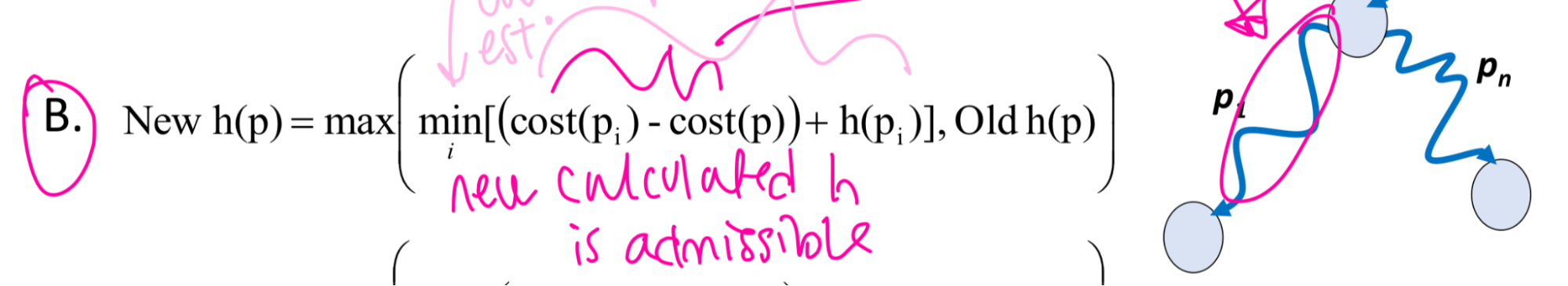
• MBA*
  • Updating the heuristic for an ancestor of multiple paths ^^^
  • Time complexity: O(b^m)
  • Space complexity: O(b^m)
  • Optimal, complete

Lecture 6

Lecture 7

• Heuristic: estimate of minimum distance/cost from each node to goal node
• Construct admissible heuristics
  • Never an overestimate of the minimum cost from n to a goal
  • Lower bound
  • Make problem extremely easy to solve
• Verify heuristic dominance
  • h2 > h1, h2 is better because its bigger and so closer to actual value
• Combine admissible heuristic
  • h = max(h_1,h_2) also admissible and dominates both h_1 and h_2

Lecture 8

Lecture 9

• Cycle checking: prune a path that ends on node already in path
  • Cannot remove optimal solution
• Dynamic programming:
  • Build of table of dist(n) - dist(n) is actual cost of lowest cost path from node n to goal g

Lecture 10

• Variables
  • Number of possible worlds: product of cardinality of each domain
  • Always exponential in number of variables
  • domain^variables
• Constraints
  • Unary
  • kary
• CSP
  • Consists of set of variables, domain for each variable, set of constraints

Lecture 11

• Generate and test
  • Brute force, generate all possible worlds one at a time and test for violations
  • Runtime: number of world
  • Can solve any CSP
• Search
  • Every solution at depth n, heuristic not useful
  • Search space: finite without cycles
  • DFS with pruning
  • Efficiency depends on order in which variables assigned values -> degree heuristics
• Consistency
  • Prune domain as much as possible before searching
  • Constraint network
• Arc consistency
  • An arc <X, r(X,Y)>: for each x in dom(X), there is a y in dom(Y) such that r(x,y) satisfied
  • Remove value in domain if not satisfied

Lecture 12

• Arc consistency algorithm
  • Order of considering arcs does not affect final output
  • May need to prune variable domain to make arc consistent
• Max number of constraints for binary: (n*(n-1))/2 (n variables)
• How many times same arc inserted into todoarc list: d (number of elements)
• How many steps to check consistency of arc: d^2
• Constraints: O(n^2)
• Overall time complexity: O(n^2d3)

• Domain splitting
  • When domains have more than one value
    • Apply DFS with pruning
    • Split the problem into two or disjoint cases
      • Set of solutions is union of solution sets
      • Need to keep around many constraint networks

Midterm 2

Lecture 13

• Local search on CSP
  • Start from possible world
  • Generate some neighbors
  • Move to neighbor and repeat steps
  • No frontier
• Constrained optimization
  • Interactive best improvement: select neighbor that optimizes some evaluation function -> minimum number of constraint violations
• Scoring function to solve CSP by local search through greedy descent or hill climb
  • Hill climb: maximizes value based function
  • Greedy descent: minimize cost based function
  • Problems: local maxima, plateaus and shoulders

Lecture 14

• Stochastic local search
  • Alternate between
    • Hill climbing
    • Random steps
    • Random restart
  • Random steps:
    • One step: choose (variable, value) pair
    • Two step: pick variable then value
  • Good in local settings, repair with minimum number of changes
  • No guarantee to find solution even if one exists can stagnate
    • Very hard to analyze
    • Not able to show no solution exists
• Comparing SLS algorithms
  • SLS algorithms are randomized
  • Taken time to solve problem is random variable

Lecture 15

• Tabu list
  • Maintain a tabu list of the k last nodes visited
• Simulated annealing
  • Change degree of randomness over time
    • Start high then low
    • If n’ better than n move, otherwise move maybe depending on temperature
    • Higher the T, more likely to move to n’ if it is worse than n
  • If T decreases slowly enough, then simulated annealing search will find a global optimum with probability approaching 1
• Beam search
  • Maintain popular of k individuals
  • Parallel search:
    • Running k random restarts in parallel rather than in sequence
  • Choose best k out of all the neighbors
  • Non stochastic beam search: lack of diversity
  • Stochastic: selects k individuals at random but probability of selection proportional to their value h(n)
• Genetic algorithm
  • Start with k randomly selected individuals
  • Fitness function
  • Successors generated by combining two individuals
    • Selection
    • Crossover
    • Mutation
  • Slow

Lecture 16

• State: full assignments
• Goal: agent wants to be in possible world where some variables are given specific values
• Successor function
  • Actions take agent from one state to another
• Solution
  • Sequence of actions that take agent from current state to goal state
• STRIPS
  • Action has
  • Precondition:
    • Set of assignments to features that mush be satisfied in order for action to be legal
  • Effects
    • Set of assignments to features that are caused by the action
  • All features not explicitly set by action stay unchanged
• Forward planning
  • States are possible worlds
  • Arcs represent actions that are legal in state s
    • Possible actions are those preconditions are satisfied in s
  • Plan is path from the state representing the initial state to a state that satisfies the goal

Lecture 17

• Heuristic for forward planning
  • Estimate of distance (cost) from a state to the goal
  • (number of actions)
• Features are binary
• goals/preconditions can only be assignments to T
• Most sense as admissible heuristic: number of unsatisfied goals -> remove all negative effects
  • Removing preconditions (trivialize)
  • Assuming no action can achieve more than one goal (inadmissible)
• Empty-delete list
  • Remove all effects that make variable false -> emptying the delete list
  • Solve simplified planning problem
• Planning as CSP
  • Unroll the plan for fixed number of steps -> horizon
  • With a horizon of k
    • Construct CSP variable for each STRIPS variable at each time step from 0 to k
    • Construct boolean CSP variable for each STRIPS action at each time step from 0 to k-1
    • Construct CSP constraints corresponding to start and goal values, as well as preconditions and effects of actions
    • Initial constraints: constrain state variables at time 0
    • Goal constraints: constrain state variables at time k

• Actions cannot simultaneously (action constraint)
  • Mutual exclusion
• State constraint
  • Hold between variables at the same step
  • Capture physical constraints
• CSP returns shortest solution

Lecture 18

• Atom: symbol starting with lowercase letter
• Body is atom or is of form b^b
• Definite clause is atom or rule of the form h <- b
• Knowledge base: set of definite clauses

Lecture 19

• Interpretation assigns a truth value to each atom
  • A possible world
• b1 ^ b2 is only true of b1 is true in I and b2 is true in I
• Rule h <- b is false in I only if b is true in I and h is false in I
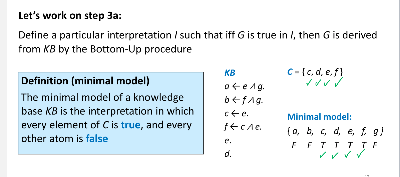
• Knowledge base KB is true in I if and only if every clause in KB is true in I
• Model of a set of clauses (a KB) is an interpretation in which all the clauses are true
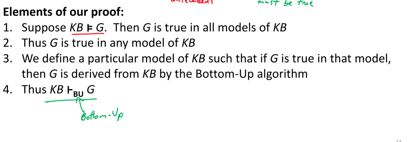
• If KB is a set of clauses and G is a conjunction of atoms, G is a logical consequence of KB, written KB |= G, if G is true in every model of KB
  • If KB true then G true
  • G logically follows from KB
  • KB entails G
  • No interpretation in which KB is true and G is false
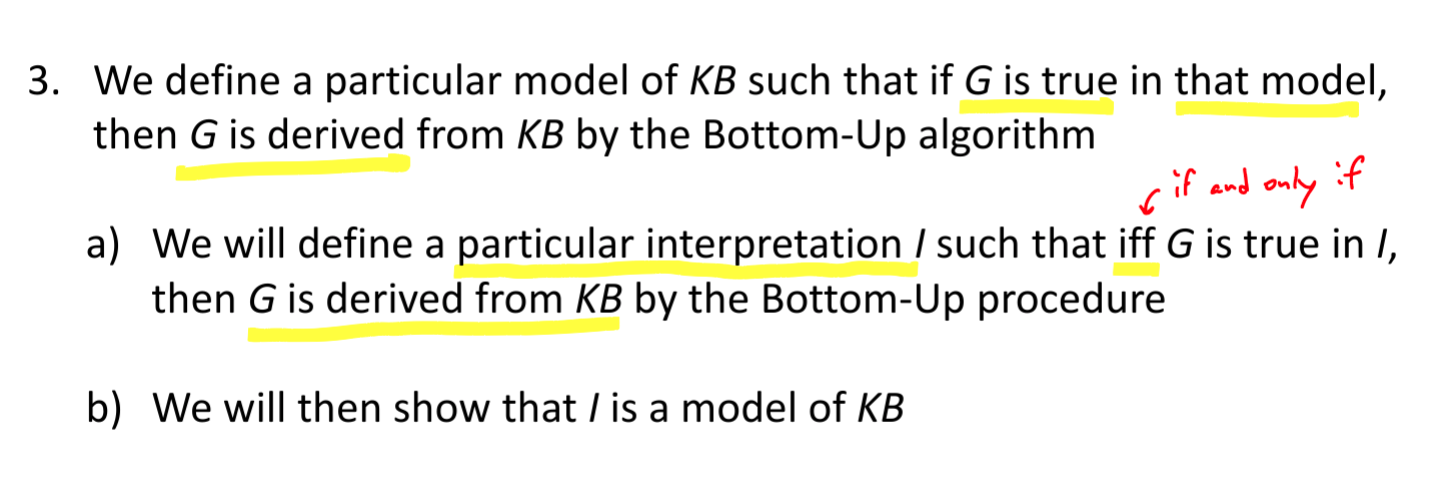
• To prove KB |= G
  • Collect of models of KB
  • Verify that G is true in all those models
  • O(2^n) time
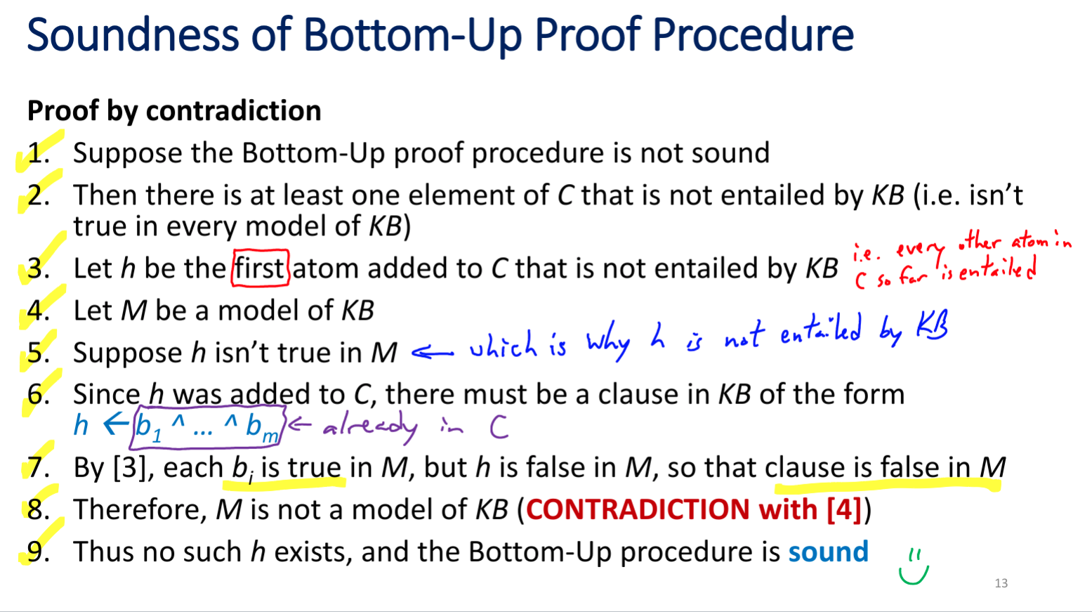
• Soundness: if KB |- G implies KB |= G (G can be derived from my proof)
• Completeness: if KB |= G implies KB |- G
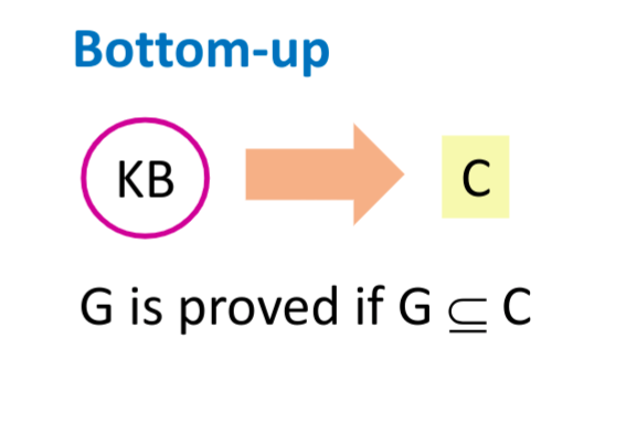
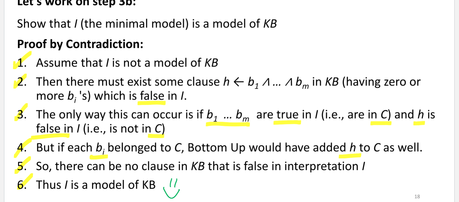
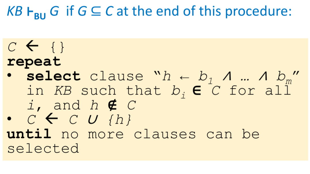
• Bottom up proof
  • If h <- b1 ^ b2 ^ b3 is a clause in the knowledge base, and each bi has been derived, then h can be derived

Lecture 20

• Given domain with n propositions, you have 2^n interpretations

Lecture 21

• Sound: never wrong
• Complete: doesn’t miss anything

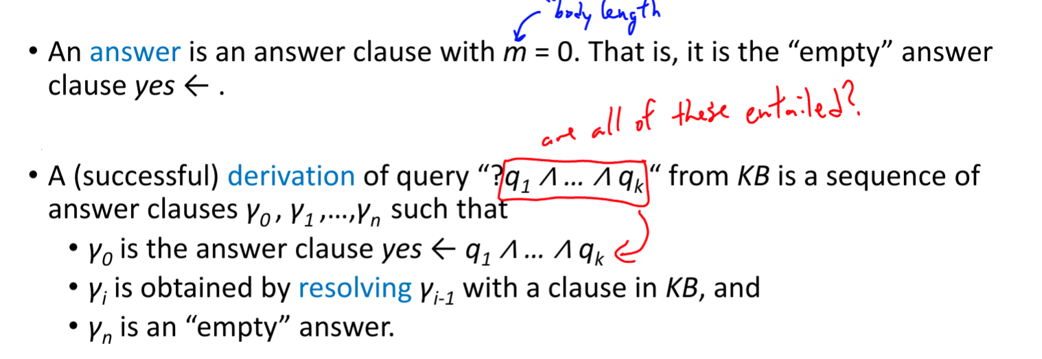
• Top down proof example

• BU looks at query G at the end

Lecture 22

• Heuristic for clause selection
  • Number of unique atoms in KB clause body

• Variable: symbol starting with an uppercase letter
• Constant: symbol starting with a lower-case letter or a sequence of digits
• Term: either a variable of a constant
• Predicate symbol: symbol starting with a lower-case letter
• Atom: symbol of form p or p(t1…tn)
• Definite clause: h <- b1^…bm
• Knowledge base: set of definite clauses

Lecture 23

• Domain of random variable X is set of values X can take
  • Values are mutually exclusive and exhaustive
• Possible worlds are mutually exclusive and exhaustive
• Joint probability distribution
  • Can compute probability distribution of any variable
  • Can compute probability distribution for any combination of variables
  • Can update these probabilities

Lecture 24

• Probabilistic conditioning
  • update/revise beliefs based on new information
  • Build probabilistic model using background information -> prior information
  • Posterior probability of h: P(h|e) -> probability of h given e
• Computing conditional probability
  • When some worlds are ruled out, others become more likely
    • Must normalize new world’s probability
    • Old probability / probability evidence
  • P(h^e)/P(e) = P(h|e)
• Conditional probability table: each row sums to 1
  • Is a set of distributions
• Product rule
  • P(x1,x2) = P(x2)(Px1|x2) = P(x1)P(x2|x1)
    • Communitive
  • P(x1, x2, …, xn) = P(x1…xt, xt+1,…xn) = P(x1…xt) P(xt+1…xn | x1…xt)
• Chain rule

• Using conditional probability for inference
  • Often have casual knowledge -> P(symptom | disease)
  • Want evidential reasoning -> P(disease | symptom)
• In general P(hypothesis | evidence)
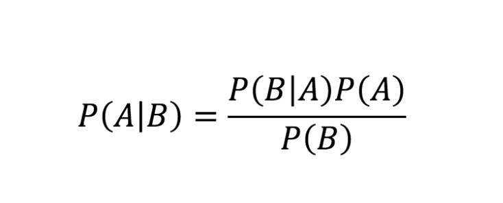
• bayes rule

Lecture 25

• Marginal independence
  • A variable x is marginally independent of random variable Y if P(x|y) = p(x)
  • P(X|Y) = P(X)
  • P(Y|X) = P(Y)
  • P(X,Y) = P(X)P(Y)
• Conditional independence
  • Each event caused by the same event, but neither event has a direct effect on the other
  • Two variables might not be marginally independent, but can become independent when we observe some third variable
  • P(X|Y,Z) = P(Y|Z)
  • Knowledge of Y’s value does not affect your belief in the value of X, given a value of Z
    • If we don’t know Z, Y and X effect each other, otherwise they don’t/q
  • P(X, Y,Z) = P(X|Z)
  • P(Y, X,Z) = P(Y|Z)
  • P(X,Y|Z) = P(X|Z)P(Y|Z)
• Joint probability distribution: O(d^n) values
  • But they have to sum to 1
  • Need to store all but 1
• Conditional probability table O(d^n) values
  • But each row has to sum to 1 (set of distributions)
  • Need to store all - (num rows)
  • Ignore a column
• Conditional independence use
  • Write out full JD using chain rule
  • Reduce JD from exponential in n to linear in n (n is # of variables)
  • Most basic and robust form of knowledge about uncertain environments
• Big picture
  • JPD specified probability of every world
    • Reduce the size with independence (rare) and conditional independence (frequent)

Lecture 27

• Belief networks
  • Order reflects causal knowledge (causes before effects)
  • Apply chain rule
  • Simplify according to marginal and conditional independence
  • Express remaining dependencies as a network
  • Each variable a node
  • For each variable, conditioning variables are its parents
  • Associate with each node the corresponding conditional probabilities
  • Result is DAG
• Bnet inference types
  • Diagnostic: know the result
  • Predictive: know cause
  • Inter-causal: one possible cause and effect
  • Mixed:
• Bnet compactness
  • O(n2^k) for n variables and each variable has no more than k parents